Background
When a person later found to have COVID-19 may have exposed people living on a unit (such as a floor of a hospital or long term care home), infection prevention and control (IPAC) measures are implemented to reduce the risk of transmission among infected people on that unit. This is done to prevent morbidity and mortality from COVID-19, but the risk of COVID-19 is also balanced by the harms of the IPAC measures themselves, such as the loneliness and physical deconditioning that can result from preventing visitors and restricting residents to their rooms. The probability that an undetected case of COVID-19 is present on a unit following possible exposures is therefore a key figure in determining when lift certain IPAC measures.
Here, we propose a method to estimate the probability of an undetected case of COVID-19, when a given number of people have been exposed, with a given pretest probability of having COVID-19 as a result of that exposure. Since we are interested in undetected COVID-19, we assume no person has developed symptoms (which would warrant further investigation) and that everyone was tested with polymerase chain reaction (PCR) on a given day, and all tested negative.
Presence of COVID-19 on the unit
To identify the congregate setting following a suspected exposure event, several assumptions and determinations must be made
- Estimate the pretest probability for each exposure
- Assume the exposure events are independent
- Determine the date of the exposure (or last possible date) to set as
Day 0.
Empirical data are required:
- What is the sensitivity and specificity of the test available, by day since exposure?
- What is the distribution of the incubation period (for symptomatic cases) in the target population?
- What proportion of cases are asymptomatic in the target population?
Methods
pretest probability
The initial pretest probability (at Day 0) of each exposed resident following exposure or possible exposure is specified by the investigator. The initial pretest probability is the expected probability the individual will develop COVID-19.
Here, we are not considering the scenario where a resident’s pretest probability increases due to the presence of symptoms. The goal of this tool is to aid the decision of when to test and when to ease restrictions if all exposed remain asymptomatic and no cases are detected.
The incubation period of COVID-19 has been modeled by several groups and a meta-analysis pooled 8 studies to estimate a lognormal distribution of the incubation period [@mcaloonIncubation2020] with mu 1.63 (1.51, 1.75), sigma 0.5 (0.45-0.55).
plot(0:21, dlnorm(0:21, 1.63, 0.5),
     xlab="Days after exposure",
     ylab="Probability",
     main="Incubation period",
     type = "b")
First ignoring asymptomatic individuals, we can calculate the daily pretest probability for those who do not develop symptoms.
plot(0:21, plnorm(0:21, 1.63, 0.5),
     ylab="Proportion",
     xlab = "Days since exposure",
     main="Infected expected to have developed symptoms",
     type="b")
The proportion of cases that are asymptomatic will vary depending on patient population. Further, the empirical data may be limited by undetected cases in ecological studies. With respect to nursing home residents, a meta-analysis found that 27.9% remained asymptomatic through follow up (Yanes-Lane et al. 2020).
plot(0:14, sapply(0:14, prop_remaining, asympt = 0.279, mu = 1.63, sigma = 0.5),
     ylab="Proportion remaining", xlab = "Day", ylim = c(0,1), type = "b")
With each passing day, if no one develops symptoms, even without testing, the pretest probability is lowered in proportion to the number of people who would have been expected to develop symptoms by that time.
plot(0:14, c(0.13, adjust_pretest(pre0 = 0.13, asymp = 0.279, days = 14)),
     ylab="pretest probability", xlab="Day", type = "b", ylim = c(0, 0.2))
Sensitivity
To account for the changing sensitivity of the PCR COVID-19 test, we used the PCR sensitivity values from a model derived from empirical data in a meta-analysis (Kucirka et al. 2020), as reported at [https://github.com/HopkinsIDD/covidRTPCR].
plot(sens$point, ylim=c(0,1),
     main="PCR Sensitivity with 95% CI",
     xlab="Days since exposure", ylab="Sensitivity",
     type="l");
lines(sens$lower, col="grey")
lines(sens$upper, col="grey")
Posttest Probability
Posttest probability can be calculated from the estimated pretest probability and the sensitivity and specificity of the test. Here, we assume a 100% specificity, and use the day-by-day sensitivity plotted above to calculate the posttest probability if testing occurred on each day, to determine the optimal day to test.
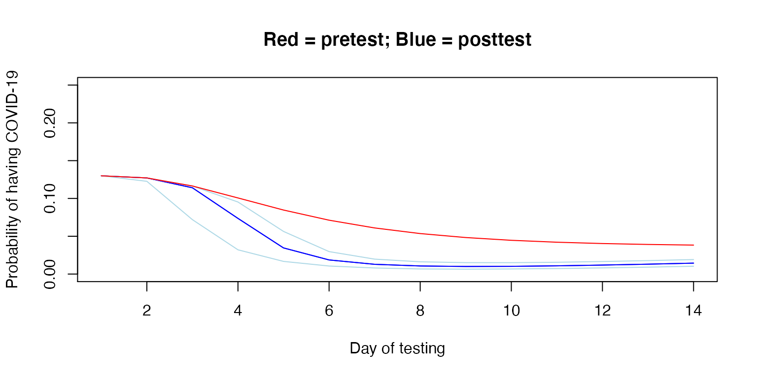
Below, we demonstrate the posttest probabilities on an example person with a 13% pretest probability at exposure and assuming 27.9% of patients in this setting remain asymptomatic.
example <- posttest_series(pre0 = 0.13, asympt = 0.279,
                           sens = sens$point, spec = 1)
example_upper <- posttest_series(pre0 = 0.13, asympt = 0.279, sens = sens$upper,
                                 spec = 1)
example_lower <- posttest_series(pre0 = 0.13, asympt = 0.279, sens = sens$lower,
                                 spec = 1)

plot(example$x, example$y,
     xlab="Day of testing",
     ylab="Probability of having COVID-19",
     main="Red = pretest; Blue = posttest",
     ylim=c(0, 0.25), col="blue", type="l")

lines(example$x, example$y,
      col="blue", type="l")
lines(example_lower$x, example_lower$y,
      col="lightblue", type="l")
lines(example_upper$x, example_upper$y,
      col="lightblue", type="l")
lines(1:14, adjust_pretest(0.13, asympt = 0.279),
      col="red", type="l")
Unit-wide posttest Probability
The relevant risk in deciding whether to maintain heightened precautions on a unit is the probability that any person is infected, or alternatively, the complement of the probability that no person is infected. That is, the probability of any case being present, is 1 less the additive probability of each case not being present.
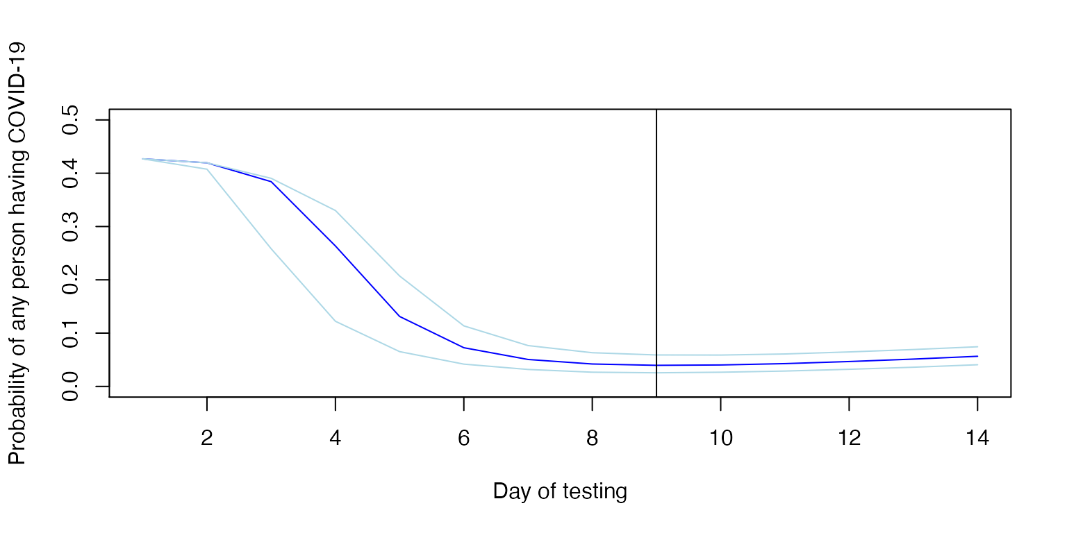
Below, we determine the posttest probability of any person having undetected COVID-19 by day, if all people were tested on the same day. Note again that the x-axis reflects the date of testing.
unit_size <- 4

any_example <- probability_any(unit_size, example$y)
any_example_upper <- probability_any(unit_size, example_upper$y)
any_example_lower <- probability_any(unit_size, example_lower$y)

plot(example$x, any_example,
     xlab="Day of testing",
     ylab="Probability of any person having COVID-19",
     ylim=c(0, 0.50), col="blue", type="l")
lines(example_lower$x, any_example_lower,
      col="lightblue", type="l")
lines(example_upper$x, any_example_upper,
      col="lightblue", type="l")

abline(v=example$x[example[,2]==min(example$y)])
In the above example, testing on day 9 yields the lowest overall posttest probability; it is the minimum. If we specify the date of testing, we can calculate and plot the change in estimated probability over time, with dates prior to testing reflecting pretest probability on that day and dates after testing reflecting posttest probability, again assuming no one develops symptoms.
test <- individual_probability(test_day = 9, pre0 = 0.13, sens = sens, spec = 1,
                               asymp = 0.279, days = 14, mu = 1.63, sigma = 0.5)

plot(1:14, test$point, type="l", ylim=c(0,0.3),
     main = "Individual probabiltiy of undetected COVID-19",
     xlab = "Days since exposure",
     ylab = "Probability")
lines(test$lower, type="l", col="grey")
lines(test$upper, type="l", col="grey")
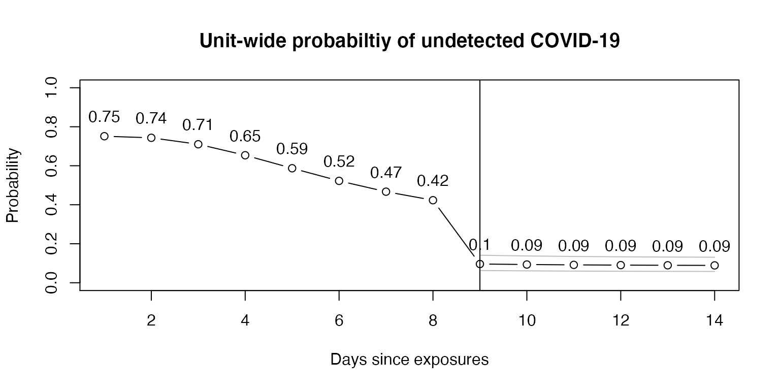
Now, using the above example, we assume there were 10 exposures and calculate the unit-wide probability of an undetected COVID-19 infection over time, again assuming all were tested on day 9.
test_n <- unit_probability(test_day = 9, pre0 =  0.13, sens = sens, spec = 1,
                           asympt = 0.279, days = 14, mu = 1.63, sigma = 0.5,
                           n = 10)

plot(1:14, test_n$point, type="b", ylim=c(0,1),
     main = "Unit-wide probabiltiy of undetected COVID-19",
     xlab = "Days since exposures",
     ylab = "Probability")
lines(test_n$lower, type="l", col="grey")
lines(test_n$upper, type="l", col="grey")
abline(v = 9)
text(1:14, (test_n$point + 0.1), round(test_n$point, 2), cex = 1)
In this example, testing on day 9 reveals a unit-wide posttest probability of 10% on day 9 and 9% when testing on day 9 and waiting until day 14. Using the lower 95% confidence interval for test sensitivity, a conservative approach, and testing on day 9, the unit-wide estimate is 14% on day 9 and 13% on day 14.
test_n$point[9]
#> [1] 0.09605053
test_n$point[14]
#> [1] 0.08898011

test_n$lower[9]
#> [1] 0.1410912
test_n$lower[14]
#> [1] 0.1309287
Discussion
Limitations and Assumptions
The results produced by this package are based on estimates and have several assumptions which may mean that it is not suitable for a given setting. This package should not be relied upon for clinical decisions, but may be useful to explore the possible relationship between certain parameters and the probability of undetected COVID-19 in a setting, acknowledging the assumptions made.
Parameters
The parameters of the model are themselves also estimates. The estimates depend on empirical data which were generally compiled from different settings. The underlying data may not apply to the setting to which the calculator is applied. This may be particularly true, for example, as emerging variants of COVID-19 impact the parameters needed for the calculations.
The distribution for the incubation period is pooled from various sources and only the point estimate of the distribution is used here. McAloon et al. report a lognormal distribution (mu = 1.63, sigma = 0.5). Lauer et al. report a similar distribution (mu = 1.621, sigma = 0.418).
The varying sensitivity of PCR tests is a pooled Bayesian estimate (Kucirka et al. 2020), and various assumptions were made to determine this best estimate, as described by the authors. Even if accurate, the test characteristics at a given site would be different than a pooled average.
The user-specified parameters are inherently estimates as well.
Pretest probability could be approximated by looking at average attack rates in certain settings with certain types of encounters. The nature of the encounter and timing of the case’s infection are important factors (https://www.publichealthontario.ca/-/media/documents/ncov/main/2020/09/covid-19-contact-tracing-risk-assessment.pdf?la=en).
The rate of true asymptomatic infections appears to vary by setting and have considerable heterogeneity. For example, at 27.9% (13.0 - 49.8%) in nursing home residents and 58.8% (48.8 - 68.1%) in obstetrical patients presenting to hospitals (Yanes-Lane et al. 2020).
Model assumptions
The model herein assumes that no exposed individuals have developed symptoms (and assumes that those who do have been identified). However, the model can be agnostic to symptoms if the proportion of asymptomatic individuals is set to 1.
The model assumes that exposures were independent events.
Future Directions (and Contributing)
This R package and accompanying Shiny app are available to the public for review. Any corrections or improvements can be recommended by filing a Github issue. As further research is done into COVID-19, improved estimates of the parameters may become available and can be incorporated into this tool.
References
Kucirka LM, Lauer SA, Laeyendecker O, Boon D, Lessler J. Variation in False-Negative Rate of Reverse Transcriptase Polymerase Chain Reaction–Based SARS-CoV-2 Tests by Time Since Exposure. Annals of Internal Medicine. 2020;173(4):262-267. https://dx.doi.org/10.7326/M20-1495
A. Lauer S, H. Grantz K, Bi Q, et al. The Incubation Period of Coronavirus Disease 2019 (COVID-19) From Publicly Reported Confirmed Cases: Estimation and Application. Annals of Internal Medicine. Published online March 10, 2020. https://dx.doi.org/10.7326/M20-0504
McAloon C, Collins Á, Hunt K, et al. Incubation period of COVID-19: a rapid systematic review and meta-analysis of observational research. BMJ Open. 2020;10(8):e039652. https://dx.doi.org/10.1136/bmjopen-2020-039652
Yanes-Lane M, Winters N, Fregonese F, et al. Proportion of asymptomatic infection among COVID-19 positive persons and their transmission potential: A systematic review and meta-analysis. PLOS ONE. 2020;15(11):e0241536. https://dx.doi.org/10.1371/journal.pone.0241536